| Home | Revision | A-Level | Economics | Theory of Production & Costs | An introduction to produc.. |
An introduction to production theory and costs
Production theory underlies all the theory of the firm, it is related to resource allocation, and it is where we get the supply curve from.
We assume for simplification:
A one-product firm.
We can identify land, labour and the units of capital used, as well as costs. Land, labour and capital are homogeneous, which means they are all identical. Firms aim to maximise profits. Other models do exist, e.g. sales maximisation,
but they are not a part of central economic theory.
Profits
Profits are not a dirty word!
But what some people will do for profit can be very dirty indeed! It is alleged that the Mafia in the USA will give you a cheap quote for removing and dealing with your toxic waste - then they might just tip it into reservoirs to get rid of it, and not spend the
money to do it properly.
The function of profits: (what are they for?)
Profits are a signal - a high rate of profit in an industry is a signal that society values that particular good or service highly and will pay a lot to get it. This tells us that more resources should go into this industry that society values so much. Individual firms move in to get the profit and as a result, resources automatically go where they are needed. Adam Smith was the first to see how a market economy allocates resources and publicise it; and this process was what he meant by “the invisible hand”.
Losses are a signal that too much is being produced, that is, output should be reduced. This means that firms ought to leave that industry, as society does not value that good or service so highly. Where profits are falling in an industry, it often means that demand has altered away from that good or service. The lower profits encourage some business people to move out.
The law of diminishing returns says that if one factor of production is increased, while holding all other factors constant, then after a point, the additions to output will start to fall and ultimately total output will decrease.
As an example, if you were to take your back garden and turn it to growing potatoes, you might start, say, with five people (N) plus five spades (K) and your garden (L).
The resulting output may be 100 kg p.a. of King Edward’s potatoes.
If you add a 6th person output (but no more spades or land) output might increase to
180 kg – the new person can weed or water while the others dig, etc., so output will rise. The addition to total output is then180-100 or 80 kg. This is the marginal product of the sixth person.
If you add a 7th person, output would still increase, perhaps to 250 kg – the addition to total output is 250-180 or 70 kg, which is the marginal product of the seventh person.
You can see the 70 kg just added is less than the 80 kg added earlier - i.e., the addition to total output from last person employed is falling, which is to say that returns are diminishing.
You might object that these figures are merely invented – which is true. But think! By the time you get to the 200th person, standing in your back garden and only five spades to work with, output is not going to be large! It is probably zero, in that there is no room to plant, dig or anything as your garden is wall-to-wall people! At some earlier point, output must have reached a maximum then fallen to nothing.
The point where output was at maximum might have been around the fifteenth or twentieth person, and after this, more people began to be a nuisance. The new person might start to gossip and distract the others; or perhaps they trip over the new comer now and then, so that output actually fell a little after he was employed. When total output starts to fall, the marginal addition is negative, and total output starts to decrease at that point.
This law must hold – we can always add enough labourers to completely fill your garden, however large, and leave no room for growing potatoes at all. The same applies
to producing anything, for example, T-shirts. The table below shows a possible scenario.
SEEING THE LAW OF DIMINISHING RETURNS TO THE FACTOR OF PRODUCTION LABOUR
| Workers per day |
Output – T-shirts per day |
Marginal product (T-shirts per worker) |
Average product (T- shirts per worker) |
|---|---|---|---|
| 1 | 2 | 3 by (subtraction from col. 2) | 4 (col. 2 ÷ col. 1) |
| 0 | 0 | ||
| 1 | 4 | 4 (4-0) | 4.00 |
| 2 | 10 | 6 (10-4) | 5.00 |
| 3 | 13 | 3 (13-10) | 4.33 |
| 4 | 15 | 2 (15-13) | 3.75 |
| 5 | 16 | 1 (16-15) | 3.20 |
| 6 | 14 | -2 (14-16) | 2.66 |
| 7 | 11 | -3 (11-14) | 1.57 |
You should observe that in the above table:
1. As we add labour, total product increases.
2. Marginal product rises at first, then falls steadily after that, and finally it becomes negative.
3. When the marginal product is above the average product, average product is increasing; when marginal product is below the average product, average product is decreasing.
This is the property of averages, it has nothing to do with economics! When the amount added exceeds the average, it must pull the average up.
Let’s take an example of a Premier League soccer team week by week and see the
average, total and marginal scores
Soccer Match: Average, Total, and Marginal Goals Scored
| Match Number | Goals scored in match |
Total goals scored (adding col. 2) |
Average goals per match (col. 3 ÷ col. 1) |
Marginal goals per match (col. 2) |
|---|---|---|---|---|
| 1 | 2 | 3 | 4 | 5 |
| 1 | 2 | 2 | 2.00 | 2 |
| 2 | 4 | 6 | 3.00 | 4 |
| 3 | 1 | 7 | 2.33 | 1 |
| 4 | 0 | 7 | 1.75 | 0 |
| 5 | 3 | 10 | 2.0 | 3 |
If you examine the table you will see that when the margin is above the average, it pulls the average up. And when the margin is below the average, it starts to pull it down.
It not only applies to a team scoring goals, or indeed any set of figures, it works just the same way in production. We can graph this too!
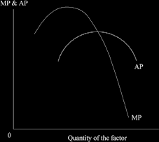
As a firm adds labour, we can show the changes in marginal product (MP) and average product (AP) in a diagram.
So looking at the T-shirt example the soccer scoring table you will see that the information on totals, marginals and averages follows a similar pattern.
The average product and the marginal product curves
We can also draw a diagram of the total product curve.
The total product curve
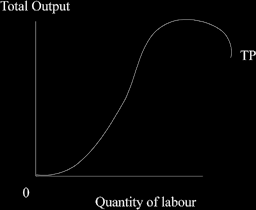
Why is it that shape?
Before we hire any labour there will be no output, so the curve starts at the origin.
At first, it is easy to produce, we can get the necessary workers and staff we need easily, and so the output curve increases and also accelerates upwards.
Later on, we will start to encounter problems, so the growth in output slows, then reaches a peak, and finally will fall.
What sort of problems might be encountered? They could be things like:
We will start to run out of machinery (remember that we are only increasing labour, holding other factors constant) so that the relationship between the number of workers and the number of machines gets worse. In simple terms, the balance is wrong. In the example of your garden, the workers ran out of spades and had to find something else to do you will recall.
The emergence of bottlenecks in the factory – storage space for materials, semi- finished and finished products perhaps.
Possibly the workers cannot find parking space nearby, which annoys them, and they then feel disgruntled and lower their efforts. This would not be the law of diminishing returns as such, but a loss of motivation.
The production function
The production function shows how many of the factors of production we must use to get various different levels of output. In other words, it shows the relationship between different inputs and the resulting output.
We can see production function in several ways:
1. We can see it in the generalised form
O = f (L, N, K) + R
(Which means “Output is related in some way to the inputs of land, labour, capital and the catch-all remainder term”).
2. We can see it as the total product curve above. In the diagram, as we increase the use of labour, we can watch total product increase. This is a simple, one factor model.
3. We can also see it as a box of choices, using two factors of production labour and capital.
The production function as a box of choices
One question is how can we produce using the resources we have got? How shall we combine them? (this is called “the choice of technique”).
The firm could use:
1) A lot of capital and a little labour; or
2) A lot of labour and little capital.
Engineering information gives us the figures in the box that might look like: The Box of Choices
| Capital (across) Labour (down) |
1 machine | 2 machines | 3 machines | 4 machines |
|---|---|---|---|---|
| 1 worker | 9 | 18 | 26 | 33* |
| 2 workers | 20 | 27 | 33* | 38 |
| 3 workers | 26 | 33* | 38 | 42 |
| 4 workers | 33* | 39 | 42 | 45 |
| 5 workers | 35 | 41 | 44 | 46 |
You can see that we can produce 33 units of output in several different ways – the firms will choose the cheapest method or the choice of technique to use, to maximise profits.
If wages are low (relative to the cost of machines) the firm would use as more workers and fewer machines - four workers and one machine would do it (this is typical of a developing country like Indonesia).
If wages are high (relative to the cost of machinery) the firm would choose to use more machines and few workers – in this case two machines and one worker (this is typical of a rich developed country like the UK or USA).