An introduction to efficiency

There is some overlap with Unit 2 about efficiency, so some of this you may already know.

The types of efficiency in economics:

a) Allocative efficiency. b) Productive efficiency.

This concept of efficiency is static. Static efficiency looks at given resources and tries to get the most output from them – and all firms should sell at a fair price to consumers, which would reflect the real resources used.

A. Allocative efficiency

This occurs when the value the consumer puts on a good or services is identical with the cost of resources used in producing it. This happens when price = marginal cost. In this situation, total economic welfare is maximised.

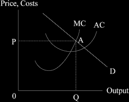
At A, with P2 and Q2, MC = P we have allocative efficiency.

In the perfect competition diagram below, where MC = MR for the firm, we have allocative efficiency because firms marginal revenue is the price, so MC = P.

The consumer surplus and the producer surplus

You will recall these concepts which were introduced in Unit 1. If you have forgotten, go back and look it up now, before reading on.

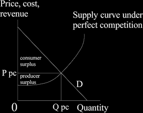
Here we are in perfect competition with price “P pc” and quantity “Q pc”.

There is allocative efficiency in a perfectly competitive industry and price equals marginal cost.

Note that the whole of the area between the supply curve and the demand curve is taken up by the consumer surplus and the producer surplus.

This is not the case in the monopoly diagram below. In contrast, in that diagram that area is not all taken up by the two surpluses. You can see the triangle of “dead weight loss” that goes neither to consumer surplus or producer surplus and so is lost to

society! We do not have allocative efficiency (where MC=MR) because the monopolist limits output and sells at a higher price in order to maximise profits.

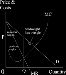
The deadweight welfare loss under monopoly is the small triangle as indicated.

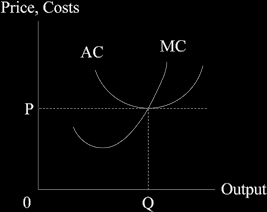
B. Productive efficiency

This kind of productivity exists when we are on the production frontier; this means we are using the least resources possible to produce any given output. This also means that we are at the minimum point on the AC curve.

This happens when we are in perfect competition – so economists prefer this state and may refer to as it “X-efficiency” – it is where we are truly efficient.

Where market equilibrium is efficient, we cannot make someone better off without making someone else worse off (this is sometimes called “the Pareto optimum position”).

Note that we can have allocative and productive efficiency but still have inequity. As an example, if you as an individual have all the income in the suburb in which you live, the other people living there will be poor and might even starve! The market system is amoral i.e., it is not concerned with good or bad.

Social efficiency matter too!

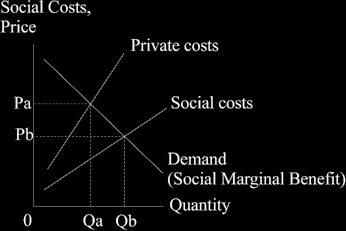
We might produce too much or too little for our own good as a society, even if have perfect competition and an acceptable distribution of income. This can happen because of the existence of externalities. The state might intervene and try to encourage all positive externalities and reduce the negative ones.

Recall the discussion in Unit 2 about externalities, social costs, and private costs. If you are less than certain about these, now would be a good time to go back and revise that part of the course.

Here as a reminder are the two diagrams involved.

Negative externalities cause the social cost curve to be above the private cost curve.

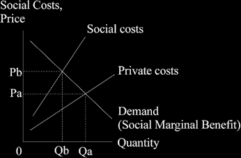
Positive externalities (usually harder to find) cause the social cost curve to be below the private one.

This temporary old revision section will automatically redirect to new version once ready.