Consumer and producer surplus

We know that there is an equilibrium market price at which both consumers buy and suppliers sell. But what about the consumers and producers who are not themselves exactly at that equilibrium price? They receive a benefit.

For consumers, we can see from the demand curve that the first consumer, buying at 1 on the quantity axis, would be willing to pay P1, which is much more than the market price he or she has to pay (P mkt). So the column above P mkt is a sort of surplus that the first buyer enjoys!

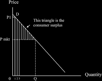
Similarly, for the second buyer, at 2 on the quantity axis; and the same goes for the third and subsequent buyers until we get out to Q1 and P Mkt. All these early consumers would pay more but do not have to do so - and they gain a lot of extra enjoyment as a result. Eventually the whole triangle above P Mkt is filled in; and the filled in bit of this triangle, indicated by an arrow, is the consumer surplus.

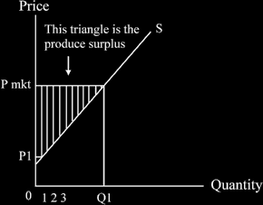
For producers, we have an analogous argument. Some would be willing to supply more cheaply than the equilibrium price, P Mkt. In the diagram below, we can see from the supply curve that the supplier of the first unit would be happy to do this at a price well below P Mkt. The column above quantity 1 up to P Mkt is again a sort of extra or surplus - which in this case belonging to the producers.

Moving to quantity 2, again we can see a column, but a bit smaller than for quantity 1. And as we move out towards Q1, the triangle above the supply curve but below P Mkt is filled in. The arrow again points to it. This is “the producers’ surplus”.

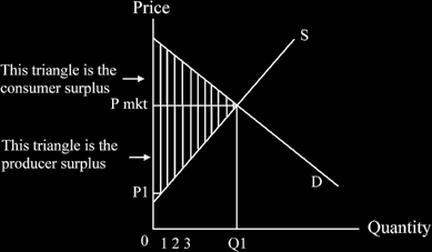
If we put the two diagrams together, we can see that both the triangles thus make up the total con- sumer surplus and the producer surplus.

Use of the concept

With indirect taxation, the imposition of a tax (or if there already is such a tax, an increase or decrease in such a tax) may impinge more on consumers than producers - or vice versa! “Who gains the most (or who loses the most)?” is the question. This may be called “the incidence of taxation”, “the tax burden”, or a question may be asked, such as “who bears the brunt of the tax?”

The answer as to who gains or loses the most depends on the elasticities involved.

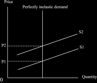
Let us assume that an indirect tax on a good increases. If demand is highly inelastic (consumers will pay almost any high price without reducing consumption much) then the increase must largely fall on these consumers - they are simply willing to pay!
We know they are prepared to do so because the demand curve is relatively inelastic and that is what inelastic demand means. Cigarettes probably fall into this category, as do all addictive drugs.

Think of a vertical demand curve: if we increase the tax, the supply curve just moves up; there is no change in the quantity demanded; suppliers still receive the old price (reading off their supply curve S1; the gap between S1 and S2 is all tax and goes to the government not to the supplier). There is clearly no loss of producer surplus as their situation has not changed at all - and consumers pay all the difference:

It can be proved, but you can take it on trust, that if the elasticity of demand is lower than the elasticity of supply, the consumer loses more than the supplier! In other words, it is the relative elasticities that count.

The usual supply and demand situation divides the incidence of tax (who pays it, or more of it) between suppliers and consumers - and of course the incidence falls heavier on the side which is relatively inelastic.
You may get a question about the incidence of tax - or one about imposing (or increasing) an indirect
tax.

A reminder: in introductory economics we nearly always use “static equilibrium analysis” which means we start in equilibrium, change something, and analyse the result.

Who then bears the burden of tax when an indirect tax increases? See the diagram below.

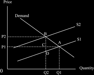
We start on the curves S1 and Demand, with the equilibrium price P1 and quantity Q1.

Then we add a tax (or increase an existing tax!) which shifts the supply curve up to S2, by the amount of the tax. Any tax per unit shifts the supply curve up vertically; the tax is the line BD in the diagram above.

Having made our change, we look at the result: consumers pay BC of the tax, and producers pay CD of it. The distance CD is smaller than the distance BC, the consumer pays more of the tax, and we also know that the elasticity of supply must be greater than the elasticity of demand!

We can also look at the areas and see the changes in both surpluses: The consumer surplus reduces by ABC.
The producer surplus reduces by ACD.

In Unit, “Industrial economics”, we again use the concept of surpluses in our monopoly diagram. We can show the deadweight loss of monopoly, as well as the loss of consumer surplus and the increase in the producer surplus that results from the monopolist being able to set the quantity that he or she pro- duces which results in the most profitable price possible. More of this later!

This temporary old revision section will automatically redirect to new version once ready.