| Home | Revision | A-Level | Economics | Labour Markets | The demand for labour |
The demand for labour
This was covered in Unit 4-1; the section here is a reminder because the marginal product curve is important – it is the demand curve for labour.
Marginal productivity theory
This gives us the demand curve for labour.
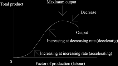
The total product curve shows us what happens to output as a firm takes on more workers With no workers, there is no output – as the firm hires one or two workers it produces some output – as it hires more people, output increases and the rate of increase is faster (output is speeding up) because there is a better balance between workers and the machinery they are using. There were too few workers at first; but eventually there will be too many workers for the machinery they have got, so the increase in output starts to slow down, then eventually output must fall.
An example: if we start growing cabbages on a football ground with 20 spades, 20 hoes, and a lorry for transport we can see that as we get more workers, one, two, three, four… and so on, output can rise rapidly.
But when we get to 1 million workers, output must have fallen to zero as the whole ground is full of people!
Marginal product = the addition to the total product from the last unit of factor added
(which is a worker in our example).
The marginal product curve rises rapidly when total product is increasing at an increasing rate (that is, the high marginal product pulls up total product rapidly); the marginal product curve falls as total product increases at a slower rate; the marginal product curve
cuts the X axis (becomes negative) when the total product is at maximum (as total product starts to fall it must mean that the marginal product being added is negative!)
Average product = total product divided by the number of workers; it is the average product per head.
We put the physical marginal product curve into money terms, by multiplying the number of units of output by the price we can sell them at. This is done so that we can compare wages (in pounds) with the marginal product (also in pounds). The curve is called the “marginal revenue product curve” or MRP.
Looking at the AP curve and the MRP curve together:
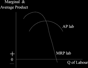
The demand curve for labour is the MRP curve (the bit below the AP curve because a firm will not pay more than a worker is worth to it on an average basis!).
Why the MRP curve? Logic! An owner will hire a worker for, say, £400 a week if s/he adds more to the firm, such as £700, or £600, or £500…. But not if s/he adds less than
£400. At the marginal product falls to £399 then the owner stops hiring. This eventually happens as we push out to the right along the horizontal Q of labour axis. The firms
stops hiring when the marginal product added is just equal to the wage that has to be paid!
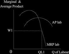
The equilibrium wage rate is set in the market for those particular workers, where supply equals demand. Any firm has to pay the going rate to get the necessary workers. The firm could chose to pay more than that, but this means it would be paying more than it needs and it would not be maximizing profits. (If it should choose to pay more to get better workers than average, then it is simply paying the market rate for the better workers!)
So the marginal revenue product curve is the demand curve for labour! At the level of the firm, we can simply read off where the market-determined wage reaches the MP curve; that then determines how many workers a firm is willing to hire.
Seeing the Law of Diminishing Returns to a Factor Making Sweaters or Jumpers
| Number of workers | Output of jumpers per day | Marginal product (jumpers per worker) | Average product (jumpers per worker) | Price of jumpers £ | Marginal revenue product £ |
|---|---|---|---|---|---|
| 1 | 2 | 3 (by subtraction from 2) |
4 (2 ÷ 1) |
5 (assumed) |
6 (3 x 5) |
| 0 | 0 | ||||
| 1 | 4 | 4 | 4.00 | 10 | 40 |
| 2 | 10 | 6 | 5.00 | 10 | 60 |
| 3 | 13 | 3 | 4.33 | 10 | 30 |
| 4 | 15 | 2 | 3.75 | 10 | 20 |
| 5 | 16 | 1 | 3.20 | 10 | 10 |
| 6 | 14 | -2 | 2.66 | 10 | -20 |
| 7 | 11 | -3 | 1.57 | 10 | -30 |
This assumes: there is perfect competition (the firms do not have to reduce price to sell more which means there is a perfectly elastic demand curve. If the firm faces a normal demand curve, it must reduce its selling price below £10 in order to increase sales, so the marginal revenue product would fall faster than if multiplied by an unchanged price of ten).
If the wage is determined in the market at £30, we can read down the marginal revenue product column and see that the firm will hire three workers. However, if the daily wage is only £20, the firm will hire four workers.
“The demand for labour is a derived demand”
People are only hired to produce something – that something is then sold. If the demand for this product or service increases then the demand for the labour to make it increases. And if demand falls, so the demand for labour falls.
Elasticity of demand for labour
This is very similar to the earlier price elasticities. The elasticity of demand for labour is measured by the percentage change in the quantity of labour demanded divided by the percentage change in the wage rate. i.e. -
% ch QlabD ÷ % ch W
The degree of elasticity depends on
1. The easier it is to substitute another input for the one we are looking at, the more elastic is demand. In other words, if it is easy to substitute capital for labour, the demand for labour is more elastic – if the wage rate goes up, firms can easily cut back on labour and use machines instead.
2. The greater the elasticity of demand for the final product, the more elastic. If the firm cannot pass on price increases, it will try to resist wage increases as it will be difficult to pass them on.
3. The greater the proportion of total costs (TC) made up by this input, the more elastic it will be. If it is a tiny percentage of TC, you can see that even a doubling in wage would not affect the final selling price much.
4. Long run elasticity is always greater than short run. This is because any needed adjustments can be made in the long term, which means a flatter (more elastic) curve. For instance, technology could be changed in order to use less labour; in the long run, whatever the firm would like to change it can.